---
title: Visualization of data distribution Linear R
tags: HowTo, CCS, Interactive, EN
GA: UA-155999456-1
---
{%hackmd @docsharedstyle/default %}
# HowTo: Visualize Your Data
## 1. Using Jupyter Notebook (Python)
### Step 1. Sign in TWCC
- If you do not have an account yet, please refer to [Sign Up for TWCC](https://www.twcc.ai/doc?page=register_account)
### Step 2. Create an interactive container
- Please refer to [Interactive Container](https://www.twcc.ai/doc?page=container#Creating-interactive-containers) to create an interactive container, and please select TensorFlow for the Image Type.
### Step 3. Connect the container
- Use Jupyter Notebook to connect to the container. Add a Python 2 notebook.
:::info
:book: See [Using Jupyter Notebook](https://www.twcc.tw/doc?page=container#Using-Jupyter-Notebook)
:::
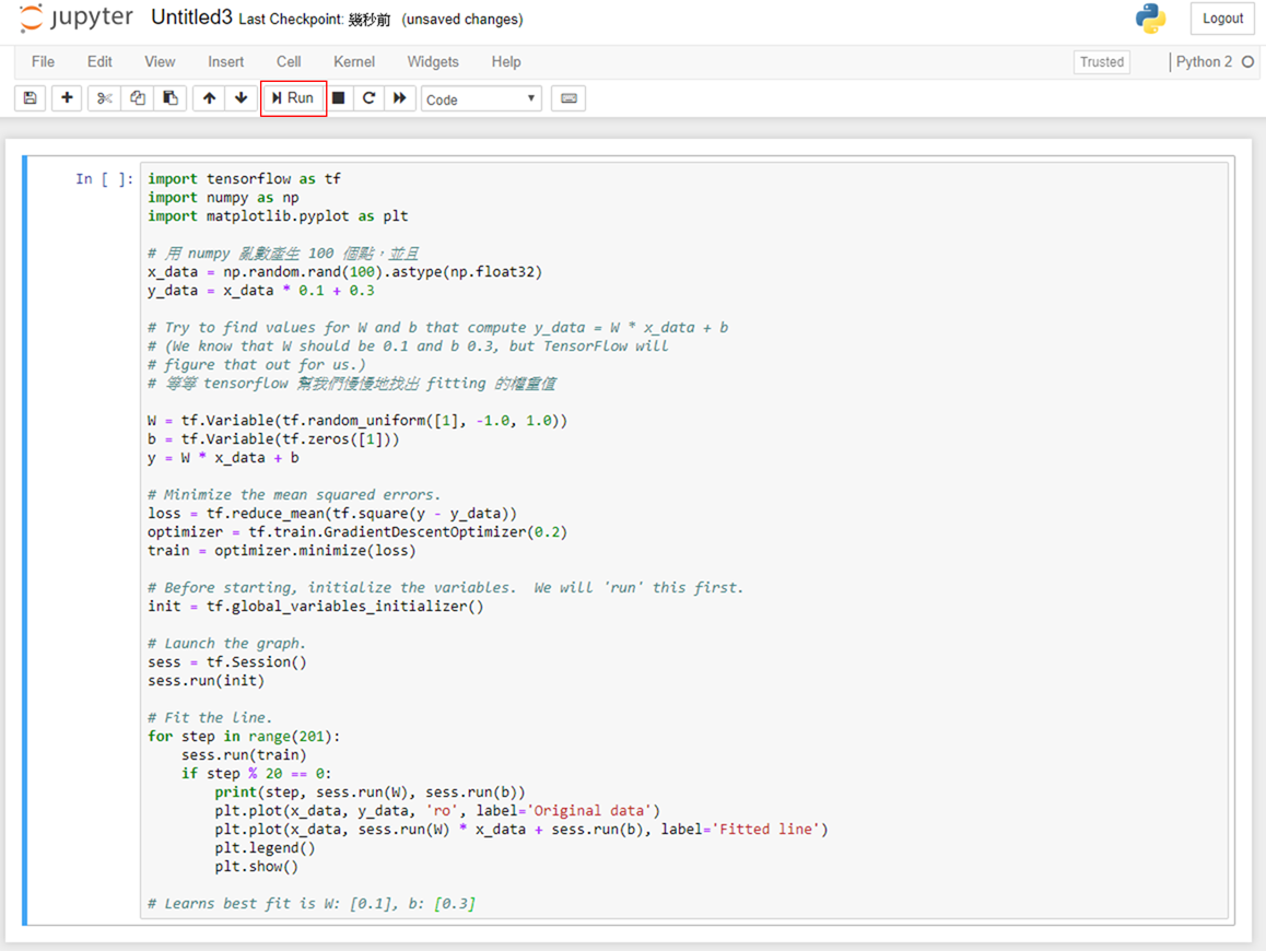
### Step 4. Execute the Linear-Regression program
- Copy and paste the following code to Jupyter Notebook
```python=
%matplotlib inline
Import tensorflow as tf
Import numpy as np
Import matplotlib.pyplot as plt
# Generate 100 points with numpy random numbers
X_data = np.random.rand(100).astype(np.float32)
Y_data = x_data * 0.1 + 0.3
# Try to find values for W and b that compute y_data = W * x_data + b
# (We know that W should be 0.1 and b 0.3, but TensorFlow will
# figure that out for us.)
W = tf.Variable(tf.random_uniform([1], -1.0, 1.0))
b = tf.Variable(tf.zeros([1]))
y = W * x_data + b
# Minimize the mean squared errors.
Loss = tf.reduce_mean(tf.square(y - y_data))
Optimizer = tf.train.GradientDescentOptimizer(0.2)
Train = optimizer.minimize(loss)
# Before starting, initialize the variables. We will 'run' this first.
Init = tf.global_variables_initializer()
# Launch the graph.
Sess = tf.Session()
Sess.run(init)
# Fit the line.
For step in range(201):
Sess.run(train)
If step % 20 == 0:
Print(step, sess.run(W), sess.run(b))
Plt.plot(x_data, y_data, 'ro', label='Original data')
Plt.plot(x_data, sess.run(W) * x_data + sess.run(b), label='Fitted line')
Plt.legend()
Plt.show()
# Learns best fit is W: [0.1], b: [0.3]
```
- Click "Run"
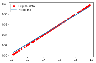
### Step 5. Visualization of data distribution
- TensorFlow will slowly find the fitting of weighted values and draw a linear regression line
:::warning
0 [-0.7029411] [0.33094117]
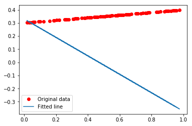
:::
.
.
:::warning
100 [0.03479815] [0.33622062]
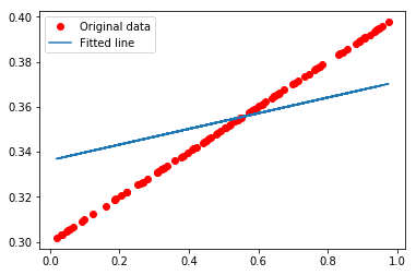
:::
.
.
:::warning
200 [0.09321669] [0.30376825]
:::
## 2. Using SSH or Jupyter Notebook (Terminal)
:::info
:bulb: The following example comes from [TensorFlow Official Tutorial](https://www.tensorflow.org/api_guides/python/regression_examples)
:::
### Step 1. Use SSH or open Jupyter Notebook (Terminal)
:::info
:book: See [How to Connect](https://www.twcc.ai/doc?page=container#How-to-connect)
:::
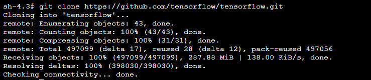
### Step 2. Download TensorFlow code from GitHub
```bash=
$ git clone https://github.com/tensorflow/tensorflow.git
```
### Step 3. Switch the Tensorflow branch to 1.10
```bash=
$ cd tensorflow && git checkout r1.10
```

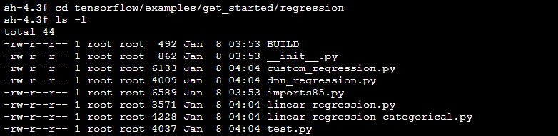
### Step 4. Switch to the example/regression directory
```bash=
$ cd tensorflow/examples/get_started/regression
```
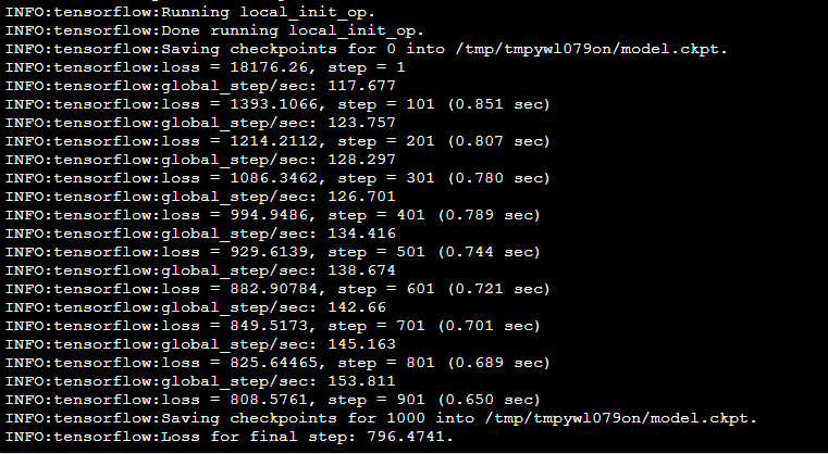
### Step 5. Run the example program using Python commands
```bash=
$ python linear_regression.py
```
- In the process of computation, the following messages will be displayed:
- Check point directory : You may use TensorBoard tool to visualize neural network and analyze training trend diagrams.
- The loss values after every 100 iterations can help examine whether it is a convergence Training.